Show some statistics of the enclosed geometric object with psydat file

import warnings

import ipywidgets as widgets
import matplotlib.pyplot as plt
import numpy as np
from ipywidgets import interact
from scipy.signal import savgol_filter

import vstt
from vstt.stats import get_velocity

/home/docs/checkouts/readthedocs.org/user_builds/vstt/envs/stable/lib/python3.11/site-packages/psychopy/preferences/preferences.py:11: UserWarning: pkg_resources is deprecated as an API. See https://setuptools.pypa.io/en/latest/pkg_resources.html. The pkg_resources package is slated for removal as early as 2025-11-30. Refrain from using this package or pin to Setuptools<81.
  from pkg_resources import parse_version

pygame 2.6.1 (SDL 2.28.4, Python 3.11.12)
Hello from the pygame community. https://www.pygame.org/contribute.html

Import

A psydat file can be imported using the psychopy fromFile function: If you want to know the detailed content of the data in psydat file, please check the notebook ‘raw_data.ipynb’

experiment = vstt.Experiment("example.psydat")
stats = experiment.stats

WARNING:root:Key 'turn_target_to_green_when_reached' missing, using default 'False'
WARNING:root:Key 'turn_target_to_green_when_reached' missing, using default 'False'
WARNING:root:Key 'area' missing, using default 'False'
WARNING:root:Key 'normalized_area' missing, using default 'False'
WARNING:root:Key 'peak_velocity' missing, using default 'False'
WARNING:root:Key 'peak_acceleration' missing, using default 'False'
WARNING:root:Key 'to_target_spatial_error' missing, using default 'False'
WARNING:root:Key 'to_center_spatial_error' missing, using default 'False'
WARNING:root:Key 'movement_time_at_peak_velocity' missing, using default 'False'
WARNING:root:Key 'total_time_at_peak_velocity' missing, using default 'False'
WARNING:root:Key 'movement_distance_at_peak_velocity' missing, using default 'False'
WARNING:root:Key 'rmse_movement_at_peak_velocity' missing, using default 'False'

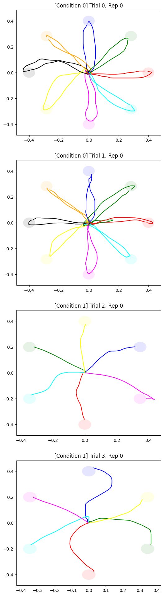
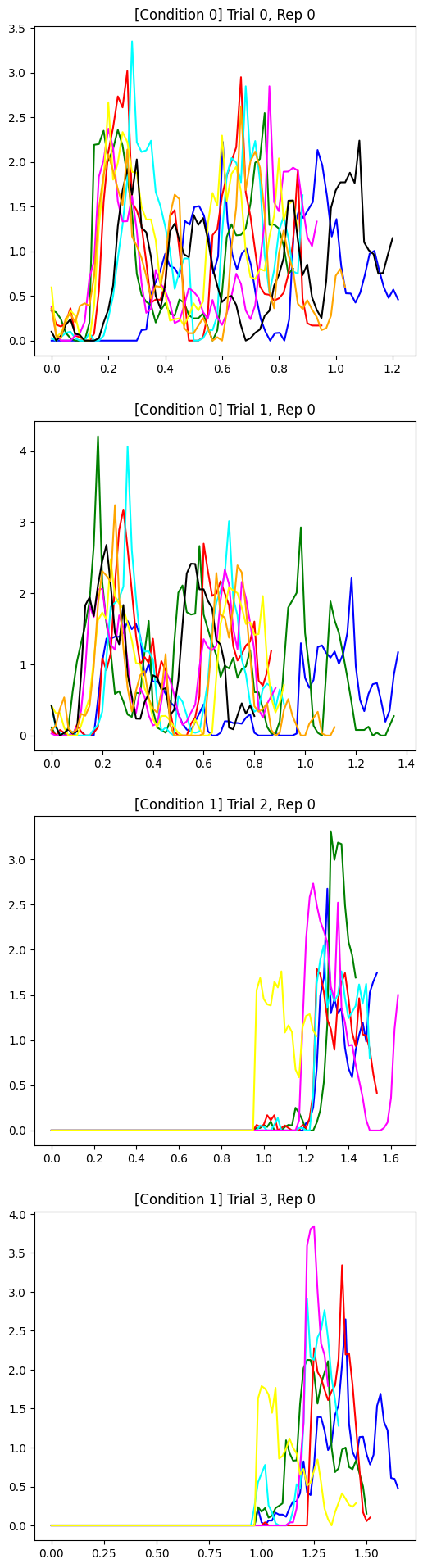
Plot of results for each trial

For example, a scatter plot of the mouse positions for each trial, labelled by the condition, trial number and repetition number:

def plot_to_target(ax, group, colors):
    for target_pos, target_radius, positions, color in zip(
        group.target_pos, group.target_radius, group.to_target_mouse_positions, colors
    ):
        ax.plot(positions[:, 0], positions[:, 1], color=color)
        ax.add_patch(
            plt.Circle(
                target_pos,
                target_radius,
                edgecolor="none",
                facecolor=color,
                alpha=0.1,
            )
        )


def plot_to_center(ax, group, colors):
    for central_target_radius, positions, color in zip(
        group.center_radius,
        group.to_center_mouse_positions,
        colors,
    ):
        ax.plot(positions[:, 0], positions[:, 1], color=color)
        ax.add_patch(
            plt.Circle(
                [0, 0],
                central_target_radius,
                edgecolor="none",
                facecolor="black",
                alpha=0.1,
            )
        )


def concatenate(array1, array2):
    return np.concatenate(
        (
            array1,
            array2,
        ),
        axis=0,
    )

colors = ["blue", "green", "red", "cyan", "magenta", "yellow", "black", "orange"]

nTrials = len(stats["i_trial"].unique())
nReps = len(stats["i_rep"].unique())
fig, axs = plt.subplots(nTrials, nReps, figsize=(6, 6 * nTrials * nReps))
axs = np.reshape(
    axs, (nTrials, nReps)
)  # ensure axs is a 2d-array even if nTrials or nReps is 1
for (trial, rep, condition_index), group in stats.groupby(
    ["i_trial", "i_rep", "condition_index"]
):
    ax = axs[trial, rep]
    ax.set_title(f"[Condition {condition_index}] Trial {trial}, Rep {rep}")
    plot_to_target(ax, group, colors)
    if not experiment.trial_list[condition_index]["automove_cursor_to_center"]:
        plot_to_center(ax, group, colors)

plt.show()

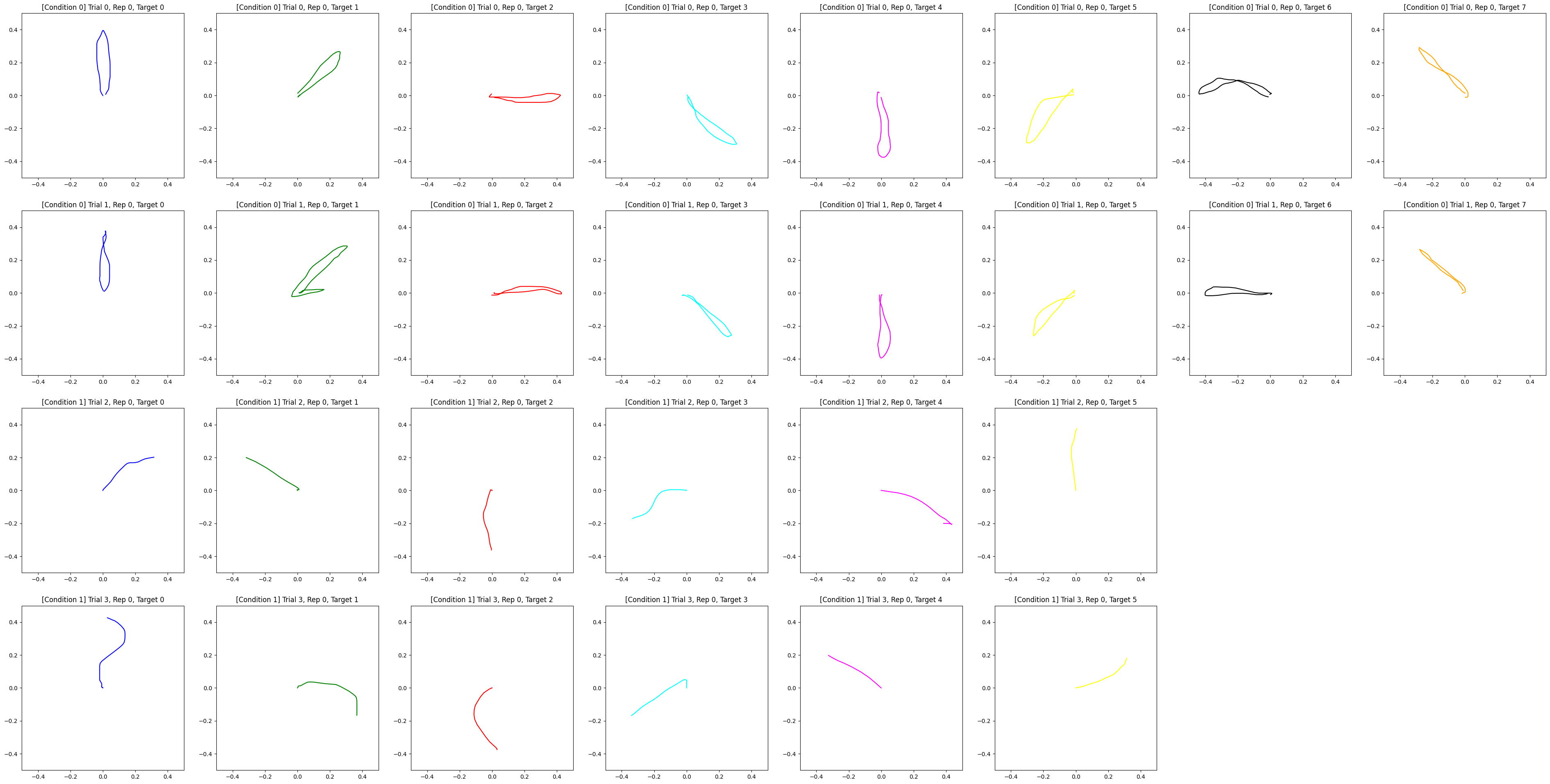
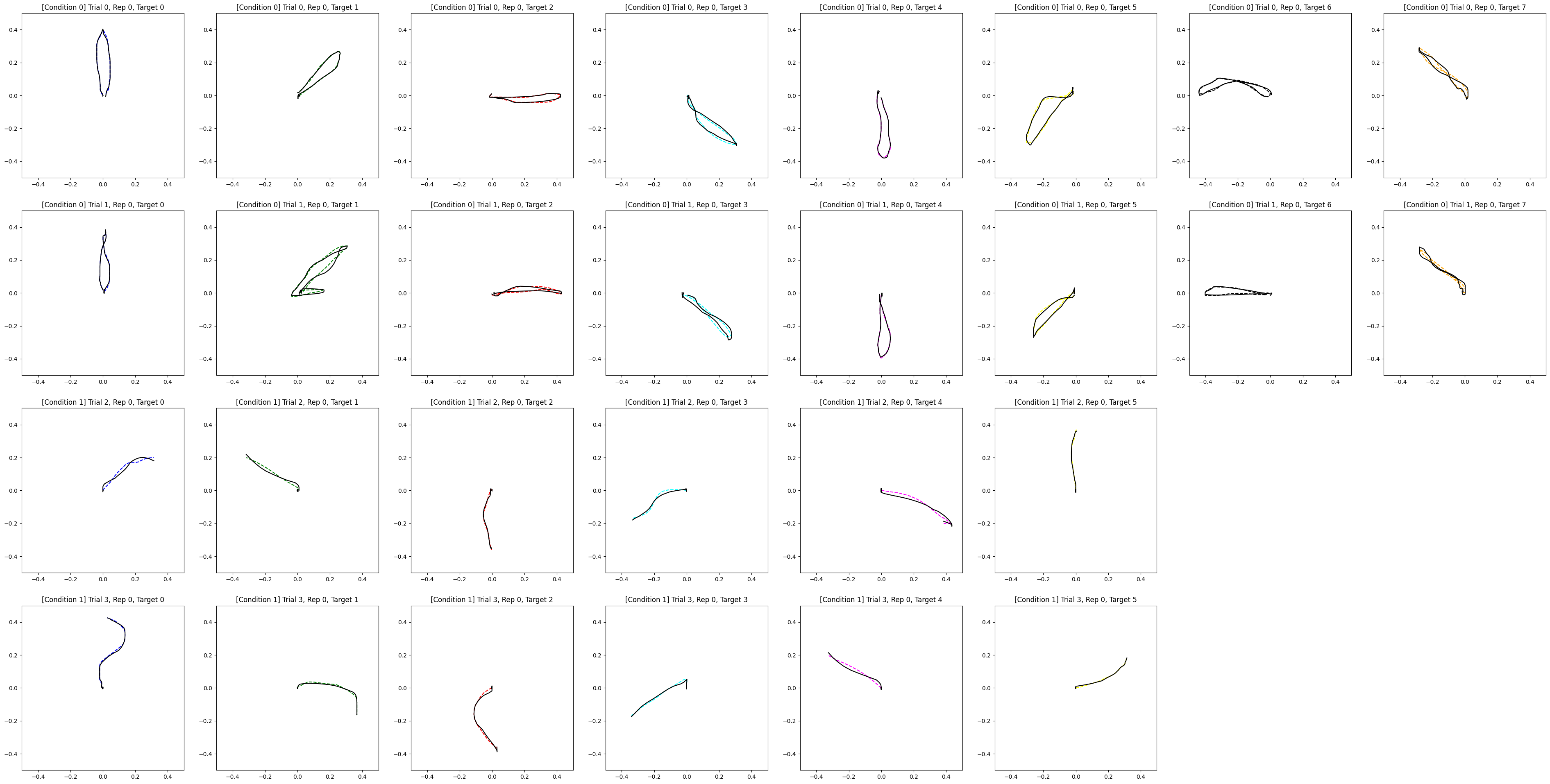
Plot of results for each target

For example, a scatter plot of the mouse positions for each target, labelled by trial number, repetition number, target number and condition:

fig, axs = plt.subplots(nTrials, nReps * 8, figsize=(6 * 8, 6 * nTrials * nReps))
axs = np.reshape(
    axs, (nTrials, nReps * 8)
)  # ensure axs is a 2d-array even if nTrials or nReps is 1
for (trial, rep, condition_index), group in stats.groupby(
    ["i_trial", "i_rep", "condition_index"]
):
    for positions, color, i in zip(
        group.to_target_mouse_positions, colors, range(len(group))
    ):
        ax = axs[(trial, rep + i)]
        ax.set_title(
            f"[Condition {condition_index}] Trial {trial}, Rep {rep}, Target {i}"
        )
        ax.set_xlim(-0.5, 0.5)
        ax.set_ylim(-0.5, 0.5)
        if not experiment.trial_list[condition_index]["automove_cursor_to_center"]:
            positions = concatenate(positions, group.to_center_mouse_positions.iloc[i])
        ax.plot(positions[:, 0], positions[:, 1], color=color)

fig.delaxes(axs[2][6])
fig.delaxes(axs[2][7])
fig.delaxes(axs[3][6])
fig.delaxes(axs[3][7])
plt.show()

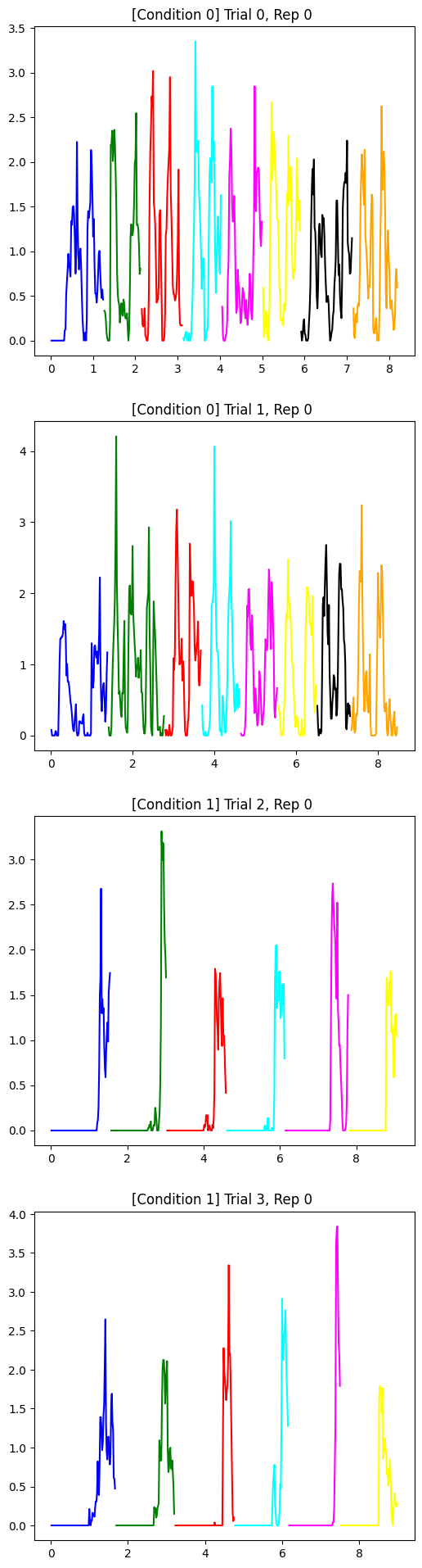
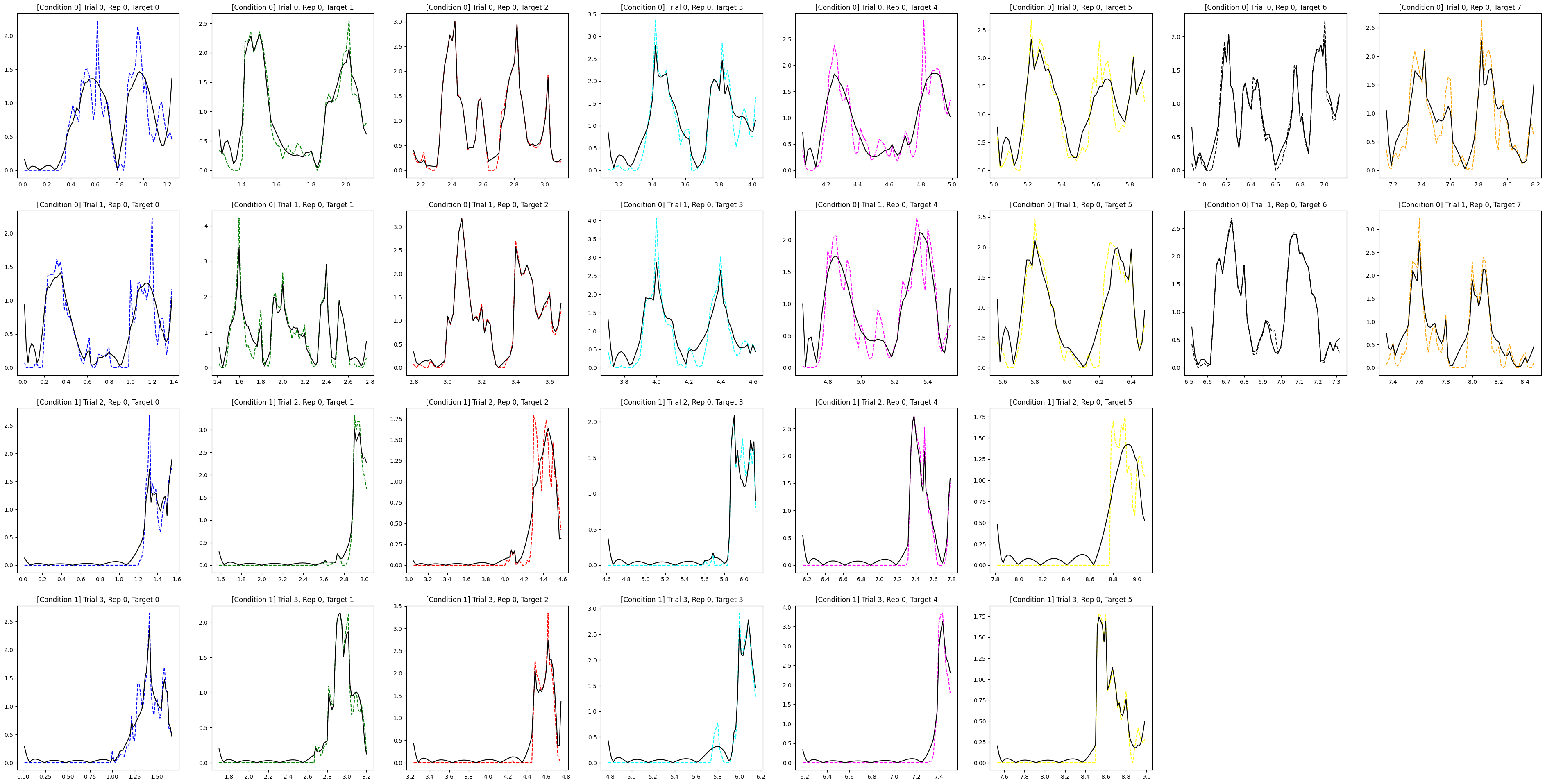
Plot velocity for each trial

For example, a scatter plot of the velocity for each target,displayed in a single plot with velocities shown in the time sequence, labelled by trial number, repetition number and condition:

fig, axs = plt.subplots(nTrials, nReps, figsize=(6, 6 * nTrials * nReps))
axs = np.reshape(
    axs, (nTrials, nReps)
)  # ensure axs is a 2d-array even if nTrials or nReps is 1
for (trial, rep, condition_index), group in stats.groupby(
    ["i_trial", "i_rep", "condition_index"]
):
    ax = axs[trial, rep]
    ax.set_title(f"[Condition {condition_index}] Trial {trial}, Rep {rep} ")
    for positions, timestamps, color, i in zip(
        group.to_target_mouse_positions,
        group.to_target_timestamps,
        colors,
        range(len(group)),
    ):
        if not experiment.trial_list[condition_index]["automove_cursor_to_center"]:
            positions = concatenate(positions, group.to_center_mouse_positions.iloc[i])
            timestamps = concatenate(timestamps, group.to_center_timestamps.iloc[i])
        ax.plot(timestamps[:-1], get_velocity(timestamps, positions), color=color)

plt.show()

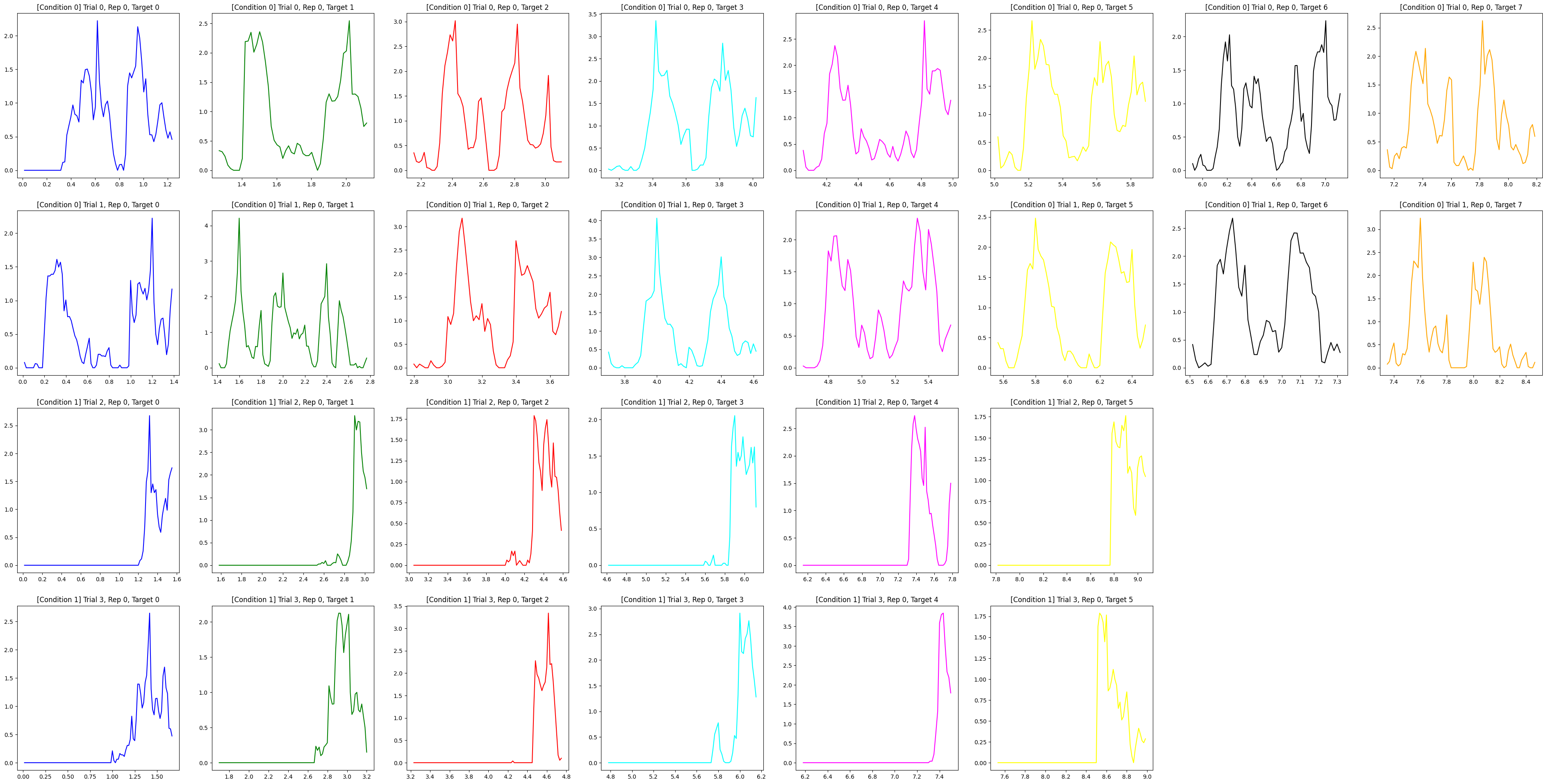
For example, a scatter plot of the velocity for each target in separate plot, labelled by trial number, repetition number and condition:

fig, axs = plt.subplots(nTrials, nReps * 8, figsize=(6 * 8, 6 * nTrials * nReps))
axs = np.reshape(
    axs, (nTrials, nReps * 8)
)  # ensure axs is a 2d-array even if nTrials or nReps is 1
for (trial, rep, condition_index), group in stats.groupby(
    ["i_trial", "i_rep", "condition_index"]
):
    for positions, timestamps, color, i in zip(
        group.to_target_mouse_positions,
        group.to_target_timestamps,
        colors,
        range(len(group)),
    ):
        ax = axs[(trial, rep + i)]
        ax.set_title(
            f"[Condition {condition_index}] Trial {trial}, Rep {rep}, Target {i}"
        )
        if not experiment.trial_list[condition_index]["automove_cursor_to_center"]:
            positions = concatenate(positions, group.to_center_mouse_positions.iloc[i])
            timestamps = concatenate(timestamps, group.to_center_timestamps.iloc[i])
        ax.plot(timestamps[:-1], get_velocity(timestamps, positions), color=color)


fig.delaxes(axs[2][6])
fig.delaxes(axs[2][7])
fig.delaxes(axs[3][6])
fig.delaxes(axs[3][7])
plt.show()

For example, a scatter plot of the velocity for each target,displayed in a single plot with velocities starting from the same time point 0,labelled by trial number, repetition number and condition:

fig, axs = plt.subplots(nTrials, nReps, figsize=(6, 6 * nTrials * nReps))
axs = np.reshape(
    axs, (nTrials, nReps)
)  # ensure axs is a 2d-array even if nTrials or nReps is 1
for (trial, rep, condition_index), group in stats.groupby(
    ["i_trial", "i_rep", "condition_index"]
):
    ax = axs[trial, rep]
    ax.set_title(f"[Condition {condition_index}] Trial {trial}, Rep {rep}")
    for positions, timestamps, color, i in zip(
        group.to_target_mouse_positions,
        group.to_target_timestamps,
        colors,
        range(len(group)),
    ):
        if not experiment.trial_list[condition_index]["automove_cursor_to_center"]:
            positions = concatenate(positions, group.to_center_mouse_positions.iloc[i])
            timestamps = concatenate(timestamps, group.to_center_timestamps.iloc[i])
        ax.plot(
            timestamps[:-1] - timestamps[0],
            get_velocity(timestamps, positions),
            color=color,
        )

plt.show()

apply a Savitzky-Golay filter example

Here is an example for illustrating how to apply a Savitzky-Golay filter to the velocity

def plot_filter(window_length, polyorder):
    """
    plot the original function and filtered function
    :param window_length: The length of the filter window (i.e., the number of coefficients). If mode is ‘interp’, window_length must be less than or equal to the size of x.
    :param polyorder: The order of the polynomial used to fit the samples. polyorder must be less than window_length.
    """
    for _, group in stats.groupby(["i_trial", "i_rep", "condition_index"]):
        for positions, timestamps in zip(
            group.to_target_mouse_positions,
            group.to_target_timestamps,
        ):
            velocity = get_velocity(timestamps, positions)
            plt.plot(timestamps[:-1], velocity, linestyle="dashed")
            filtered_velocity = savgol_filter(velocity, window_length, polyorder)
            plt.plot(timestamps[:-1], filtered_velocity)
            break
        break
    plt.legend(["original velocity", "filtered velocity"], loc="upper left")
    plt.show()


interact(
    plot_filter,
    window_length=widgets.IntSlider(min=1, max=40, step=1, value=40),
    polyorder=widgets.IntSlider(min=1, max=40, step=1, value=8),
);

apply filter to the mouse positions

For example, a scatter plot of the movement for each target in separate plots, the filtered movement is displayed in black dashed line:

fig, axs = plt.subplots(nTrials, nReps * 8, figsize=(6 * 8, 6 * nTrials * nReps))
axs = np.reshape(
    axs, (nTrials, nReps * 8)
)  # ensure axs is a 2d-array even if nTrials or nReps is 1
for (trial, rep, condition_index), group in stats.groupby(
    ["i_trial", "i_rep", "condition_index"]
):
    for positions, color, i in zip(
        group.to_target_mouse_positions, colors, range(len(group))
    ):
        ax = axs[(trial, rep + i)]
        ax.set_title(
            f"[Condition {condition_index}] Trial {trial}, Rep {rep}, Target {i}"
        )
        ax.set_xlim(-0.5, 0.5)
        ax.set_ylim(-0.5, 0.5)
        if not experiment.trial_list[condition_index]["automove_cursor_to_center"]:
            positions = concatenate(positions, group.to_center_mouse_positions.iloc[i])
        ax.plot(positions[:, 0], positions[:, 1], color=color, linestyle="dashed")
        window_length = len(positions[:, 0])
        polyorder = 8
        filtered_y = savgol_filter(positions[:, 1], window_length, polyorder)
        ax.plot(positions[:, 0], filtered_y, color="black")


fig.delaxes(axs[2][6])
fig.delaxes(axs[2][7])
fig.delaxes(axs[3][6])
fig.delaxes(axs[3][7])
plt.show()

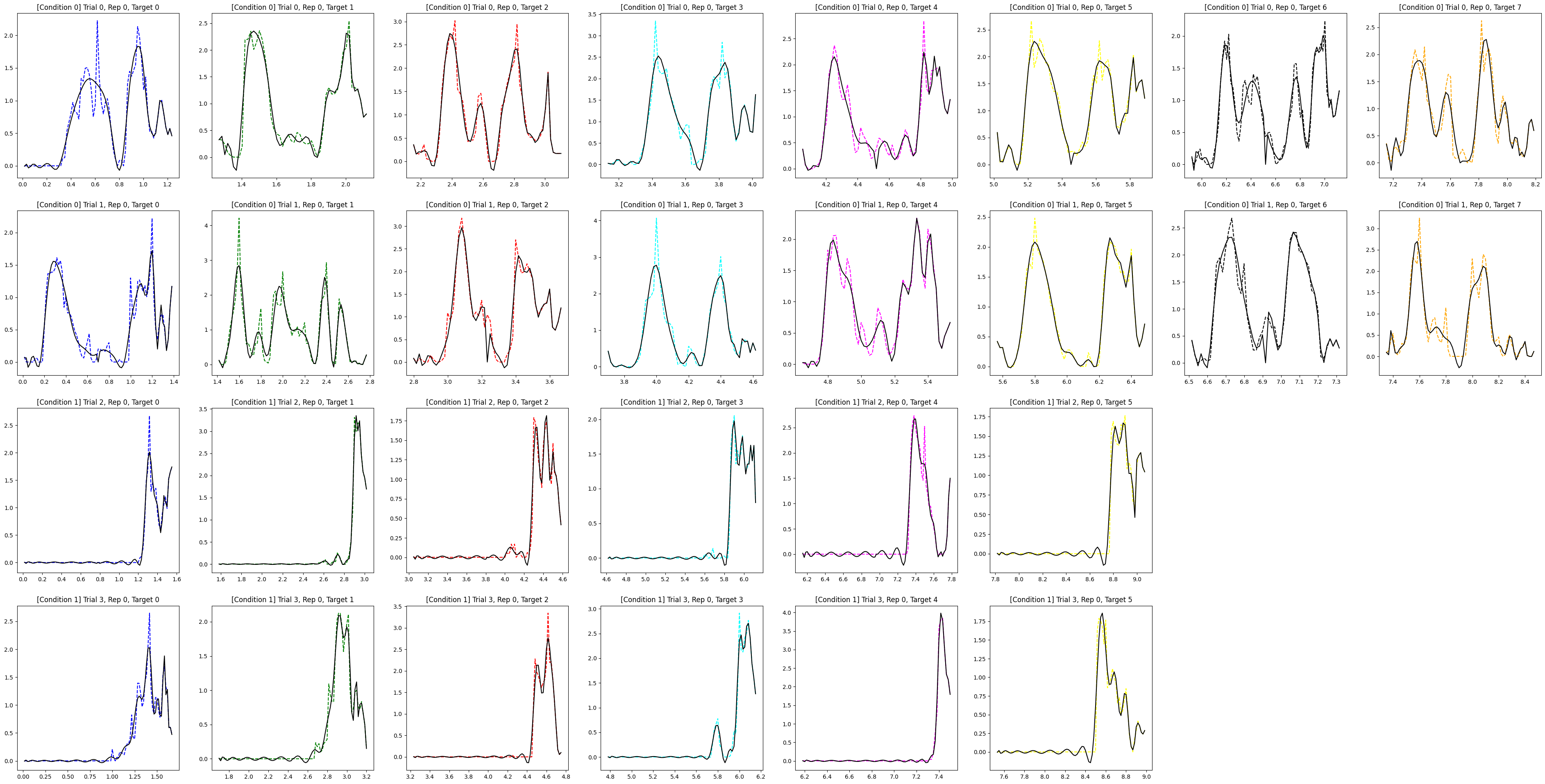
apply filter to the mouse position first, then plot the velocity

For example, a scatter plot of the velocity for each target in separate plots, the filtered velocity is displayed in black dashed line:

fig, axs = plt.subplots(nTrials, nReps * 8, figsize=(6 * 8, 6 * nTrials * nReps))
axs = np.reshape(
    axs, (nTrials, nReps * 8)
)  # ensure axs is a 2d-array even if nTrials or nReps is 1
for (trial, rep, condition_index), group in stats.groupby(
    ["i_trial", "i_rep", "condition_index"]
):
    for positions, timestamps, color, i in zip(
        group.to_target_mouse_positions,
        group.to_target_timestamps,
        colors,
        range(len(group)),
    ):
        ax = axs[(trial, rep + i)]
        ax.set_title(
            f"[Condition {condition_index}] Trial {trial}, Rep {rep}, Target {i}"
        )
        if not experiment.trial_list[condition_index]["automove_cursor_to_center"]:
            positions = concatenate(positions, group.to_center_mouse_positions.iloc[i])
            timestamps = concatenate(timestamps, group.to_center_timestamps.iloc[i])
        velocity = get_velocity(timestamps, positions)
        ax.plot(timestamps[:-1], velocity, color=color, linestyle="dashed")
        filtered_positions = positions.copy()
        window_length = len(filtered_positions[:, 1])
        polyorder = 8
        filtered_positions[:, 1] = savgol_filter(
            filtered_positions[:, 1], window_length, polyorder
        )
        velocity_with_filtered_positions = get_velocity(timestamps, filtered_positions)
        ax.plot(
            timestamps[:-1],
            velocity_with_filtered_positions,
            color="black",
        )

fig.delaxes(axs[2][6])
fig.delaxes(axs[2][7])
fig.delaxes(axs[3][6])
fig.delaxes(axs[3][7])
warnings.filterwarnings("ignore")
plt.show()

apply filter to the velocity plot to make it smoother

For example, a scatter plot of the velocity for each target in separate plots, the filtered velocity is displayed in black dashed line:

fig, axs = plt.subplots(nTrials, nReps * 8, figsize=(6 * 8, 6 * nTrials * nReps))
axs = np.reshape(
    axs, (nTrials, nReps * 8)
)  # ensure axs is a 2d-array even if nTrials or nReps is 1
for (trial, rep, condition_index), group in stats.groupby(
    ["i_trial", "i_rep", "condition_index"]
):
    for positions, timestamps, color, i in zip(
        group.to_target_mouse_positions,
        group.to_target_timestamps,
        colors,
        range(len(group)),
    ):
        ax = axs[(trial, rep + i)]
        ax.set_title(
            f"[Condition {condition_index}] Trial {trial}, Rep {rep}, Target {i}"
        )
        if not experiment.trial_list[condition_index]["automove_cursor_to_center"]:
            positions = concatenate(positions, group.to_center_mouse_positions.iloc[i])
            timestamps = concatenate(timestamps, group.to_center_timestamps.iloc[i])
        velocity = get_velocity(timestamps, positions)
        ax.plot(timestamps[:-1], velocity, color=color, linestyle="dashed")
        window_length = len(velocity)
        polyorder = len(velocity) - 1
        filtered_velocity = savgol_filter(velocity, window_length, polyorder)
        ax.plot(timestamps[:-1], filtered_velocity, color="black")


fig.delaxes(axs[2][6])
fig.delaxes(axs[2][7])
fig.delaxes(axs[3][6])
fig.delaxes(axs[3][7])
warnings.filterwarnings("ignore")
plt.show()